
Ballistic coefficient (BC) describes a bullet’s ability to overcome air resistance. It depends on the bullet’s shape, mass, and cross-sectional area. The conventional wisdom is that a higher BC is better. But anyone who accepts that without question should remember that published figures do not always tell the whole story. BC is part of a calculation method developed by Italian Francesco Siacci in 1888. The concept has been around that long. But, fear not! In this article, we will not publish equations, algorythms or formulas. Just how it works.
At the heart of the method is the accompanying table. It describes the motion of a hypothetical reference projectile with a BC of 1.0. Under the convention commonly used in the United States, this projectile weighs 453.6 grams (1 pound, or 7,000 grains) and measures 25.4 mm (1 inch) in diameter. In our example, it starts at 1,000 m/s (approximately 3,281 fps), as shown in the left-hand column.
In the next row, air resistance has slowed it to 999 m/s. The second column shows the distance traveled at that point, and the third gives the elapsed flight time. By the final row, where velocity has dropped to 100 m/s (328 fps), the projectile has traveled 10,739.9 meters (approximately 11,745 yards) in 52.6051 seconds. The Siacci table has additional columns, but these are not needed to understand the principle.
The Siacci method uses BC as a scaling factor to derive another bullet’s flight data from those of the reference projectile. One distinction matters here: the table does not describe an actual trajectory. It represents horizontal motion with gravity excluded. Air resistance is the only force acting on the reference projectile.
How ballistic coefficient is determined
To determine BC, we need to know a bullet’s velocity at two points along its trajectory. Suppose its muzzle velocity is 710 m/s (approximately 2,329 fps), falling to 641 m/s (2,103 fps) at 100 meters (109 yards). We then locate the rows for those two velocities in the table, highlighted in blue and orange.
The reference projectile, which started at 1,000 m/s, reaches 710 m/s after traveling 936.5 meters. That becomes the starting point for our comparison. The row for 641 m/s shows a distance of 1,191.8 meters. The difference, 255.3 meters, is highlighted in green: this is how far the reference projectile travels while slowing from 710 to 641 m/s. Our actual bullet loses the same amount of velocity in just 100 meters. It therefore overcomes air resistance less effectively than the reference projectile, so its BC is below 1.0. Dividing the actual distance by the corresponding distance in the table gives us its BC: 100 / 255.3 = 0.3917
Finding velocity at another distance
Let’s use 200 meters (219 yards). Because the reference projectile retains velocity better than our bullet, the corresponding distance in the table must be greater than 200 meters. Dividing 200 by our BC of 0.3917 gives a table distance of 510.6 meters, highlighted in green. We add this to our starting point of 936.5 meters, giving 1,447.1 meters. That is the table distance corresponding to our bullet’s actual flight of 200 meters. There is no entry for exactly 1,447.1 meters. It falls between the rows for 1,445.8 and 1,449.9 meters, where the velocities are 576 and 575 m/s, respectively. Interpolating between them gives a velocity of 575.7 m/s (approximately 1,889 fps) at 200 meters.
Finding the corresponding flight time
The flight times in those two table rows are 1.9073 and 1.9143 seconds. Interpolating between them gives 1.9095 seconds. This is the reference projectile’s flight time from its original starting point to 1,447.1 meters.
We subtract the 1.1123 seconds it took to reach the starting point of our comparison, leaving 0.7972 seconds. To obtain our bullet’s flight time, we multiply that interval by its BC of 0.3917. The result is 0.3123 seconds to cover 200 meters (219 yards).
So our bullet, starting at 710 m/s (approximately 2,329 fps), retains 575.7 m/s (1,889 fps) at 200 meters and reaches that distance in 0.3123 seconds. All of this requires only basic arithmetic. Notice, too, that neither bullet diameter nor bullet weight is needed for this calculation.
Understanding air resistance
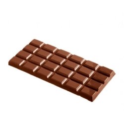
If we could isolate and weigh a cubic meter of air, it would weigh about 1.2 kilograms (2.6 pounds). That is roughly the weight of a bottle of whiskey or twelve 100-gram chocolate bars. An object moving through air must push some of that air aside, which takes force. You can feel the effect by holding your hand flat against the airflow outside a moving car’s window. The airflow produces dynamic pressure, which depends on air density and the square of velocity. Multiplying that pressure by the area presented to the airflow gives a force; the object’s shape also affects the actual drag, as we’ll see shortly. In our flat-hand example, at 50 km/h (31 mph), or 13.9 m/s, the resulting force is about 2.3 newtons.
To put the newton (N) into familiar terms, consider a 100-gram (3.5-ounce) chocolate bar. Held in your hand, it exerts a downward force of almost exactly 1 N. A force of 2.3 N therefore corresponds to the weight of about 2.3 such bars. Accelerating from 50 to 100 km/h (31 to 62 mph) produces a substantial increase in resistance. Dynamic pressure rises with the square of velocity: doubling speed quadruples it, while increasing speed tenfold multiplies it by 100. At 100 km/h, the force against the flat hand is therefore 9.2 N, four times the value at 50 km/h. Closing the hand into a fist roughly halves the area exposed to the airflow. If we account only for that smaller area, the calculated force at 100 km/h drops by half, to 4.6 N.
How shape affects drag
If we measured the drag on that fist at 100 km/h (62 mph), we would find a force of about 3.2 N rather than the calculated 4.6 N. The difference comes from shape, which also affects how air flows around an object.
We therefore need another factor: the drag coefficient, usually written as C_D in English and, in German, c_w, as the source illustrations come from a German manual. This coefficient expresses the ratio between the measured drag and the force calculated from dynamic pressure and frontal area. In our example, the flat hand has a drag coefficient of 1.0, while the fist has a value of 0.7. Multiplying the calculated force by the drag coefficient gives the actual drag: 4.6 N × 0.7 = approximately 3.2 N.
The drag coefficient cannot simply be calculated with sufficient reliability; it must be established through wind-tunnel testing or measurements of a projectile in flight. Radar has been used to track rifle bullets since the 1960s, but the measurements require high precision. In the author’s experience, inexpensive consumer radar units do not yet provide the accuracy needed for this work.
Drag coefficient changes with velocity
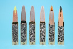
Rifle bullets travel at high velocities: a muzzle velocity of 900 m/s (approximately 2,953 fps), for example. The way air flows around a projectile changes as it accelerates or slows, so its drag coefficient does not remain constant.
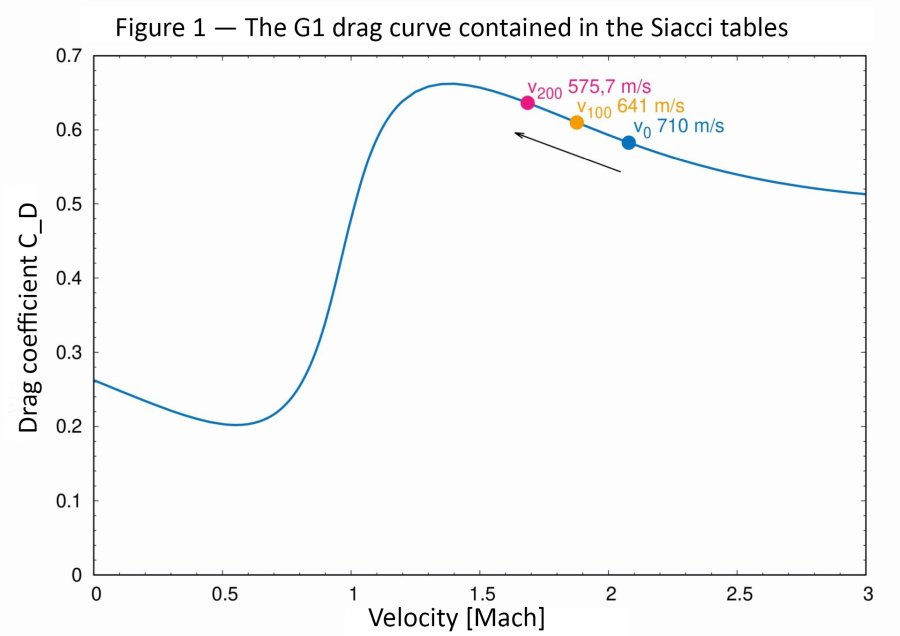
Figure 1 shows how the drag coefficient varies with velocity, ranging here from about 0.2 to 0.66. The points used in our table example are marked. Because the bullet starts fast and then slows down, we follow the curve in the direction of the arrow.
This is the G1 drag curve, which underlies many published ballistic coefficients. Although G1 reached European shooters through American usage, it originated around 1890 at the French naval proving ground at Gâvre. It also provides the drag model for the Siacci table used here.
As researchers established in the early 20th century, these changes in drag coefficient depend on the projectile’s speed relative to the speed of sound, rather than on its velocity alone. That ratio is called the Mach number. With the speed of sound at approximately 340 m/s (1,115 fps), a bullet traveling at 710 m/s (2,329 fps) is moving at Mach 2.09.
A lighter bullet slows more quickly
Under the same braking force, a fully loaded car takes longer to stop than an unloaded one. The same principle applies to bullets: with equal aerodynamic drag, the lighter bullet decelerates more rapidly. Consider a streamlined 7.62 mm (.30-caliber) bullet leaving the muzzle at 950 m/s (approximately 3,117 fps). At that velocity, it encounters about 7 N of drag. With a mass of 11.3 grams (approximately 174 grains), it travels 715 meters (782 yards) in the first second. A bullet with the same shape and dimensions but weighing only 9.45 grams (approximately 146 grains) travels 680 meters (744 yards).The lighter bullet slows more quickly under the same drag force and therefore has a lower BC. Ballistic coefficient thus accounts for two things: the aerodynamic drag acting on the bullet and the bullet’s inertia, which resists that deceleration.
Sources of error in BC calculations
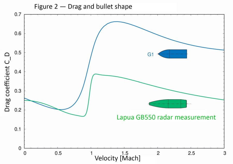
To check the method, we’ll use the radar-derived drag-coefficient tables Lapua published between 2009 and 2015. Our example is the GB550, a 7.62 mm (.30-caliber) bullet weighing 11.3 grams (approximately 174 grains). Figure 2 compares its shape and drag curve with the G1 reference projectile. Its drag is roughly half that of G1, but the more important difference is that the curves have distinctly different shapes.
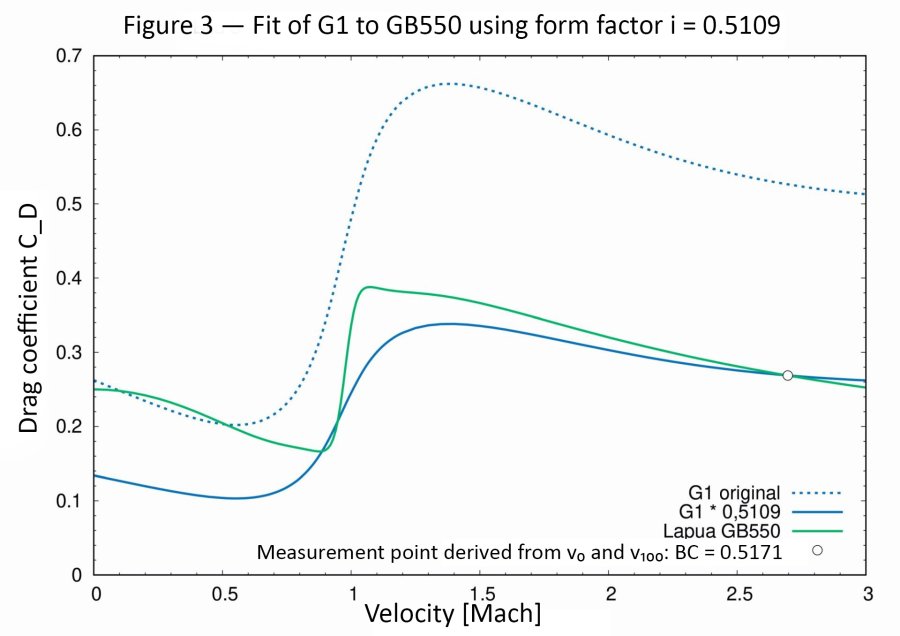
With a measured muzzle velocity of 950 m/s (approximately 3,117 fps) and a velocity of 851.2 m/s (2,793 fps) at 100 meters (109 yards), the Siacci table gives the GB550 a BC of 0.5171. That value accounts for bullet diameter and mass, as well as a form factor, designated i. Figure 3 shows what this factor does: it scales the G1 drag curve to match the measured drag.
At Mach 2.7, the GB550 has a drag coefficient of 0.2688, compared with 0.5261 for G1. Multiplying the G1 value by 0.5109 brings it down to the measured value. That multiplier is the form factor.
BC also accounts for differences in weight and diameter between the actual bullet and the reference projectile. Consequently, BC and form factor generally have different numerical values: here, BC is 0.5171 and i is 0.5109.
The method assumes that scaling the G1 curve with a form factor can reproduce the actual drag curve of a modern bullet. Figure 3 shows the limitation: even after scaling, the two curves remain substantially different.
In this example, the BC is established from velocity measurements over a short distance, between the muzzle and 100 meters. As velocity falls beyond that interval, the scaled G1 curve lies increasingly below the GB550’s measured drag curve. The calculation therefore underestimates drag, introducing an error into the predicted trajectory.
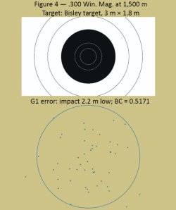
Consider a trajectory calculated to 1,500 meters (approximately 1,640 yards) using the G1 BC of 0.5171. The calculation calls for 203 clicks of elevation above the scope’s 100-meter zero. Using the GB550’s actual radar-derived drag data, however, gives 218 clicks. Each click represents 0.1 milliradian, or 1 cm at 100 meters.
As Figure 4 shows, the G1 prediction puts the shots about 2.2 meters (7.2 feet) low. In this example, none reaches the target: the bullets strike the ground roughly 50 meters (55 yards) short. The circle indicates the estimated dispersion at 1,500 meters. Designated D90, it is the circle expected to contain 90 percent of the shots.
G7 produces smaller errors than G1
Before World War II, British researchers tested more modern projectile shapes. The United States adopted two of these as G7 and G8. G8 is identical to G7 except that it lacks the boat-tail.
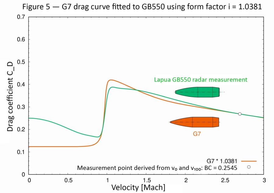
Figure 5 shows how much more closely the G7 reference projectile resembles a modern rifle bullet. Its form factor of 1.0381 is only slightly above 1, and above Mach 1, its drag curve follows that of the GB550 much more closely.
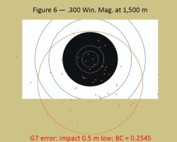
The GB550’s G7 BC is 0.2545. At 1,500 meters (approximately 1,640 yards), the resulting trajectory error is about one-quarter of the error produced by G1, as Figure 6 shows. The numerically smaller G7 BC of 0.2545 is therefore no indication of poorer performance than the G1 BC of 0.5171. BC values based on different reference drag models cannot be compared directly.
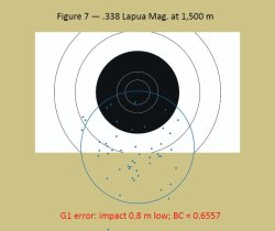
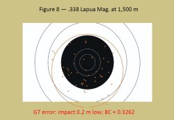
Figures 7 and 8 show the corresponding results for .338 Lapua Magnum, calculated using radar data for the 16.2-gram (250-grain) GB488 bullet.
For geometrically similar bullets, increasing diameter also increases mass relative to frontal area, giving the larger bullet greater sectional density. It retains velocity better, and errors in the drag model have less effect on the calculated trajectory.
Although the .338 Lapua Magnum’s muzzle velocity of 900 m/s (approximately 2,953 fps) is lower than that of the .300 Winchester Magnum example, its predicted points of impact are closer to the center of the target. Estimated dispersion at 1,500 meters is also smaller because flight time is shorter: 2.8 seconds rather than 3.1 seconds. Wind drift would likewise be reduced.
Conclusion: Match the drag model to the bullet and the distance
For modern, streamlined rifle bullets, G7 ballistic coefficients provide useful results, even if they are not perfect. In the examples examined here, G1 gives reasonably accurate predictions over short distances, but its limitations become increasingly apparent as range increases. The choice of reference model matters more than the size of the published number. A BC is meaningful only when we know which drag model it belongs to. If a manufacturer publishes a BC without identifying it as G1 or G7, it can generally be assumed to be G1.
As a final note, all the above is a primer just to get into the gist of BC. The depth of the rabbit hole is infinite, and the semplifications and approximations explained above are just a starting point: BC changes dynamically with speed, for example. State of the art research include multi BC charachterizations measured with enire flight travel traced with Doppler radars, and models that are much more advanced, starting with the PRODAS 6DOF and ongoing.